Damped Driven Pendulum II: Diverging Trajectories and Chaos
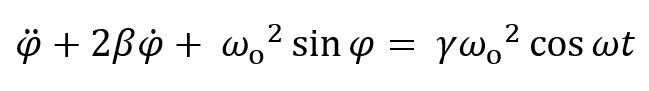
Here we go from one solution ( previous applet) to comparing two close-together solutions of the damped driven pendulum equation of motion. In the chaotic regime, we can set initial positions 10-4 radians apart, and see that the paths are apparently identical for several cycles—actually because we cannot see the exponentially increasing difference until it is a radian or so on our scale. Eventually the paths completely and randomly separate.
In nonchaotic systems, the paths usually converge, but there are exceptions. Taylor gives the example γ = 1.077 where different starting angles give different final cyclic behavior. Try this out: put γ = γ2 = 1.077, and run with φ =0, φ2 = -27 degrees, -28, -29. Compare the two curves. (Also check with different dt's: small dt and fast speed works best.)
We allow the possibility of same initial conditions, different γ. Around γ = 1.073, changes of 0.0001 dramatically alter the initial wandering before the cycle settles down. Try γ = 1.073, γ2 = 1.0731, same initial angles, vert scale 1, speed 5, horiz scale 0.4. Then, for greater precision, put dt down by a factor of 25 to 0.02 msec, speed up from 5 to 50. The transients are slightly different: this now reproduces Taylor's curve(if not, go to 0.01 msec.)
Driving strength γ = 1.105 reproduces Taylor fig 12.10: chaotic oscillation. Add γ2 = 1.106, same initial angles, and look at the result! (Take vert scale = 1.5, horiz scale = 0.5, speed = 2.)
The next applet, Damped Driven Pendulum III, plots the logarithm of the difference between the two solutions, making the exponential behavior evldent: exponential increase of separation, on average, in the chaotic regime, and exponentially falling difference in the nonchaotic case.
Here's the relevant lecture, which includes more details, and here is a link to the previous applet, which plots a single curve.
Program by: Carter Hedinger
