28. Rolling Sphere on Tilted Turntable
Michael Fowler
Introduction
We’ll now consider an interesting dynamics problem not covered in most introductory texts, a rolling ball on a rotating, possibly tilted, surface. As we’ll see, this tough sounding problem is not that difficult to solve using Newtonian methods, and leads to some surprising results. For example, a ball rolling on a steadily rotating horizontal plane moves in a circle, and not a circle centered at the axis of rotation. We’ll prove this—and demonstrate it in class. Even more remarkably, if the rotating plane is tilted, the ball follows a cycloidal path, keeping at the same average height—not rolling downhill. This is exactly analogous to an electron in crossed electric and magnetic fields. One reason the rolling ball problems are generally avoided is that they do not readily lend themselves to Lagrangian analysis, but can in fact be solved quite quickly with a vectorized application of Newton’s laws. The appropriate techniques are described in Milne’s book Vectorial Mechanics, which we follow.
Holonomic Constraints and non-Holonomic Constraints
A sphere rolling on a plane without slipping is constrained in its translational and rotational motion by the requirement that the point of the sphere momentarily in contact with the plane is at rest. How do we incorporate this condition in the dynamical analysis: the least action approach, for example, or the direct Newtonian equations of motion?
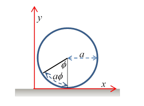
We’ll begin with a simpler example, that of a cylinder rolling in the direction, its orientation defined as zero as it passes the origin, and its radius We see immediately that its orientation is uniquely given by its position (for no slipping) by or The constraint enables us to eliminate one of the dynamical variables from the equation. If we measure its position at some later time, we know the angle it turned through. The same argument works for a cylinder rolling inside a larger cylinder.
A constraint on a dynamical system that can be integrated in this way to eliminate one of the variables is called a holonomic constraint. A constraint that cannot be integrated is called a nonholonomic constraint.
For a sphere rolling on a rough plane, the no-slip constraint turns out to be nonholonomic.
To see this, imagine a sphere placed at the origin in the plane. Call the point at the top of the sphere the North Pole. Now roll the sphere along the axis until it has turned through ninety degrees. Its NS axis is now parallel to the axis, the N pole pointing in the positive direction. Now roll it through ninety degrees in a direction parallel to the axis. The N pole is still pointing in the positive direction, the sphere, taken to have unit radius, is at
Now start again at the origin, the N pole on top. This time, first roll the sphere through ninety degrees in the direction. The N pole now points along the positive axis. Next, roll the sphere through ninety degrees in the direction: we’re back to the point but this time the N pole is pointing in the direction.
The bottom line is that, in contrast to the cylindrical case, for a rolling sphere the no-slip constraint does not allow us to eliminate any dynamical variables—given that initially the sphere is at the origin with the N pole at the top, there is no unique relationship between orientation and position at a later point, we would have to know the rolling history, and in fact we can roll back to the origin by a different route and in general the N pole will not be at the top when we return.
So the constraint equation, which can be written
does not allow us to eliminate a variable, but it certainly plays a role in the dynamics! As we've seen, the identical equation for the cylinder, , trivially integrates to uniquely linking change in orientation with change in position. We see that for a ball rolling in two dimensions, there can be no such integral.
A possible approach is to use Lagrange multipliers to take account of the constraint, just as in deriving the equation for the catenary the fixed length of the string entered as a constraint. Doing this for the rolling ball turns out to lead to a very messy problem—for once, the advanced approach to dynamics doesn’t pay off. But there’s a better way.
D’Alembert’s Principle
The “better way” is simply to write down Newton’s equations, and the rotational equivalent for each component of the system, now using, of course, total force and torque, including constraint reaction forces, etc. This approach Landau calls “d’Alembert’s principle”.
Footnote: We’re not going to pursue this here, but the “principle” stems from the concept of virtual work: if a system is in equilibrium, then making tiny displacements of all parameters, subject to the system constraints (but not necessarily an infinitesimal set of displacements that would arise in ordinary dynamical development in time), the total work done by all forces acting on parts of the system is zero. This is just saying that in equilibrium, it is at a local minimum (or stationary point if we allow unstable equilibrium) in the energy “landscape”. D’Alembert generalized this to the dynamical case by adding in effective forces corresponding to the coordinate accelerations, he wrote essentially , representing as a “force”, equivalent to Newton’s laws of motion.
Having written down the equations, the reaction forces can be cancelled out to derive equations of motion.
Ball with External Forces Rolling on Horizontal Plane
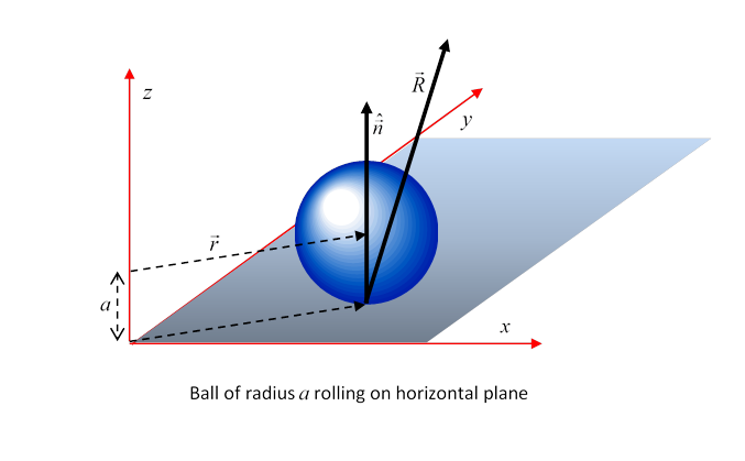
Here’s how it works for a simple example (done in Landau, and see diagram below): the equation of motion of a sphere rolling on a fixed horizontal plane under an external force and torque .
Taking the reaction at the plane to be (and note that this can be in any upward direction, not in general vertical), we have
The constraint equation, differentiated, gives so the first equation can be written then substituting from the second equation,
This equation gives the components of the reaction force as functions of the external force and couple: the velocities have been eliminated. So we can now put in the first equation of motion giving the translational acceleration in terms of the external force and torque. Note that any vertical component of the torque will not affect the reaction at the plane (it would just spin the ball about the point of contact) so we have, using ,
and substitution in the original equations of motion gives
Exercise: interpret this for the zero torque case, and for the zero force case.
Landau goes on to solve three statics problems which could be in an introductory physics course. We'll skip them.
Ball Rolling on Rotating Plane
(The following examples are from Milne, Vectorial Mechanics.)
A sphere is rolling without slipping on a horizontal plane. The plane is itself rotating at constant angular velocity .
We have three vector equations: Newton’s equations for linear and angular acceleration, and the rolling condition. We want to find the path taken by the rolling ball on the rotating surface, that is, . We’ll use our three equations to eliminate two (vector) variables: the reaction force between the plane and the ball and the angular velocity
The equations of motion of the sphere (radius mass center at measured in the lab, horizontally from the axis of the plane’s rotation) with the contact force of the plane on the sphere, are
(Of course, the gravitational force here is just balancing the vertical component of the reaction force, but this is no longer the case for the tilted plane, treated in the next section.)
First, we’ll eliminate the reaction force to get an equation of motion:
The rolling condition is:
the right-hand side being the local velocity of the turntable, measured from an origin at the center of rotation.
We’ll use the rolling condition to eliminate and give us an equation for the actual path of the sphere.
First, differentiate it (remember are both constant) to get
Next, take the equation of motion and to get
and putting these together to get rid of the angular velocity,
This integrates to
which is just the equation for steady circular motion about the point
For a uniform sphere, so
So the ball rolling on the rotating plate goes around in a circle, which could be any circle. If it is put down gently at any point on the rotating plane, and held in place until it is up to speed (meaning no slipping) it will stay at that point for quite a while (until the less than perfect conditions, such as air resistance or vibration, cause noticeable drift). If it is nudged, it will move in a circle. In class, we saw it circle many times—eventually, it fell off, a result of air resistance plus the shortcomings of our apparatus, but the circular path was very clear.
Ball Rolling on Inclined Rotating Plane
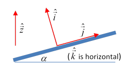
We’ll take unit vectors pointing vertically up, perpendicularly up from the plane, the angle between these two unit vectors being (We will need a set of orthogonal unit vectors not fixed in the plane, but appropriately oriented, with horizontal.) The vector to the center of the sphere (radius , mass ) from an origin on the axis of rotation, at a point above the plane, is . The contact reaction force of the plane on the sphere is
The equations of motion are:
and the equation of rolling contact is
First, we eliminate from the equations of motion to give
Note that so the spin in the direction normal to the plane is constant, say. (Both forces on the sphere have zero torque about this axis.)
Integrating,
Now eliminate by multiplying both sides by and using the equation of rolling contact
to find:
then using we find
The constant is fixed by the initial position giving finally
The first term in the square brackets would give the same circular motion we found for the horizontal rotating plane, the second term adds a steady motion of the center of this circle, in a horizontal direction (not down the plane!) at constant speed
(This is identical to the motion of a charged particle in crossed electric and magnetic fields.)
Bottom line: the intuitive notion that a ball rolling on a rotating inclined turntable would tend to roll downhill is wrong! Recall that for a particle circling in a magnetic field, if an electric field is added perpendicular to the magnetic field, the particle moves in a cycloid at the same average electrical potential—it has no net movement in the direction of the electric field , only perpendicular to it. Our rolling ball follows an identical cycloidal path—keeping the same average gravitational potential.