previous home next applets home
22a: Driven Damped Pendulum: Period Doubling, Chaos, Strange Attractors
Michael Fowler, UVa
Note: although this lecture follows naturally from the previous one (on the driven damped nonlinear oscillator), it is self-containedit does not depend on that earlier material.
Introduction
We’ve previously discussed the driven damped simple harmonic oscillator, and in the last lecture we extended that work (following Landau) to an anharmonic oscillator, adding a quartic term to the potential. Here we make a different extension of the simple oscillator: we go to a driven damped pendulum. (A weight at one end of a light rigid rod, the other end of the rod being at a fixed position but the rod free to rotate about that fixed point in a vertical plane). That is, we replace the potential term in the linear oscillator with or rather to make clear we have an angular system. Going to a driven damped pendulum leads to many surprises!
For a sufficiently weak driving force, the behavior of the driven damped pendulum is of course close to that of the driven damped linear oscillator, but on gradually increasing the driving force, at a certain strength the period of the response doubles, then, with further increase, it doubles again and again, at geometrically decreasing intervals, going to a chaotic (nonperiodic) response at a definite driving strength. But that is not the end of the storythe chaotic response regime has a lot of structure: many points within a generally chaotic region are in fact nonchaotic, well-defined cyclical patterns. And, as we’ll see later, the response pattern itself can be fractal in nature, see for example the strange attractor discussed at the end of this lecture. You can use the accompanying applet to generate this attractor and its cousins easily.
Obviously, this is a very rich subject, we provide only a brief overview. We closely follow the treatment in Taylor’s Classical Mechanics, but with the addition of our applets for illustrative purposes, and also to encourage further exploration: the applets accurately describe the motion and exhibit the strange attractors in the chaotic regime. With the applets, it is easy to check how these strange attractors change (or collapse) on varying the driving force or the damping. We end with some discussion of the fractal dimension of the attractors, and how it relates to the dynamics, in particular to the rate of divergence of initially close trajectories, here following Baker and Gollub, Chaotic Dynamics.
The Road to Chaos
Equation of Motion
For the driven pendulum, the natural measure of the driving force is its ratio to the weight Taylor calls this the drive strength, so for driving force
the drive strength is defined by
The equation of motion (with resistive damping force and hence resistive torque ) is:
Dividing by and writing the damping term (to coincide with Taylor’s notation, his equation 12.12) we get (with )
Behavior on Gradually Increasing the Driving Force: Period Doubling
The driving force is the dimensionless ratio of drive strength to weight, so if this is small the pendulum will not be driven to large amplitudes, and indeed we find that after initial transients it settles to motion at the driving frequency, close to the linearized case. We would expect things to get more complicated when the oscillations have amplitude of order a radian, meaning a driving force comparable to the weight. And indeed they do.
Here we’ll show that our applet reproduces the sequence found by Taylor as the driving strength is increased.
In the equation of motion
we therefore choose Taylor’s values and gradually increase from 0.9 to 1.0829, where chaos begins.
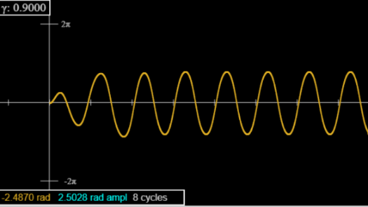
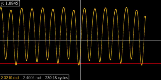
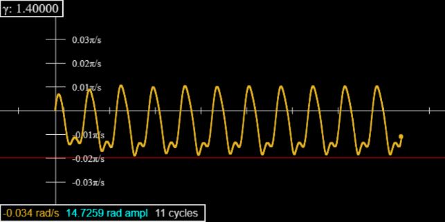
For (see picture) the oscillation (after brief initial transients) looks like a sine wave, although it’s slightly flatter, and notice the amplitude (turquoise in box) is greater than the positive and negative swings are equal in magnitude to five figure accuracy after five or so oscillations.
You can see this for yourself by opening the applet! Click here. The applet plots the graph, and simultaneously shows the swinging pendulum (click bar at top right).
For there is a larger initial transient, vaguely resembling the three-cycle we’ll meet shortly. In fact, this can be suppressed by starting at (bottom slider on the right), but there are still transients: the peaks are not uniform to five-figure accuracy until about forty cycles.
For there are very long transients: not evident on looking at the graph (on the applet), but revealed by monitoring the amplitude readout (turquoise figures in the box on the graph), the value at the most recent extremum. To get past these transients, set the applet speed to 50 (this does not affect accuracy, only prints a lot less dots). run 350 cycles then pause and go to speed = 2. You will find the peaks now alternate in height to the five-figure accuracy displayed, looks like period doublingbut it isn’t, run a few thousand cycles, if you have the patience, and you find all peaks have the same height. That was a long lived transient precursor of the period doubling transition.
Going to 1.0664, you’ll see both peaks and dips now alternating in amplitude, for a well-defined period 2, which lasts until 1.0792. (Look at 1.075 after 70 or so cyclesand set the initial angle at -90.)
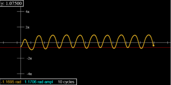
Use the “ Red Line” slider just below the graph to check the heights of successive peaks or dips.
For the period doubles again: successive peaks are now of order 0.4 radians apart, but successive “high” peaks are suddenly about 0.01 radians apart. (To see these better on the applet, magnify the vertical scale and move the red line.)
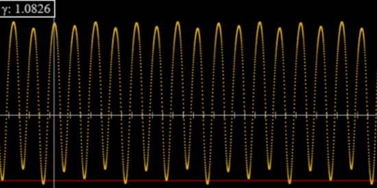
For there is a further doubling to an 8 cycle, then at 1.0827 to a 16 cycle.
Look at the graph for 1.0826: in particular, the red line near the bottom. Every fourth dip goes below the line, but the next lowest dips alternate between touching the line and not quite reaching it. This is the 8 cycle.
It is known that the intervals between successive doublings decrease by a factor found universally in period doubling cascades, and called the Feigenbaum number, after its discoverer. Our five-figure accuracy is too crude to follow this sequence further, but we can establish (or at least make very plausible!) that beyond the geometric series limit at the periodicity disappears (temporarily, as we’ll see), the system is chaotic. (Of course, the values of depend on the chosen damping parameter, etc., only the ratio of doubling intervals is universal.)
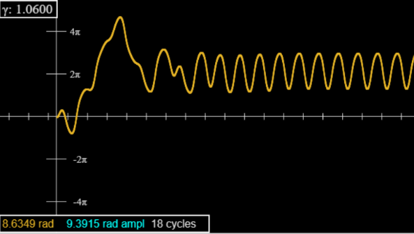
In fact, the full picture is complex: there are further intervals of periodicity, for example a 6 cycle at pictured here.
Different Attractors
The periodic solutions described above are called “attractors”: configurations where the system settles down after initially wandering around.
Clearly the attractors change with the driving strength, what is less obvious is that they may be different for different initial conditions. Taylor shows that for taking gives a 3-cycle after transients, but gives a 2-cycle. (Easily checked with the applet!)
Looking at the initial wanderings, which can be quite different for very small changes in the driving strength (compare 1.0730 to 1.0729 and 1.0731, use speed 5, it doesn’t affect the accuracy). But you can see these initial wanderings include elements from both attractors.
Exercise: use the next applet to plot at the same time 1.0729 and 1.0730, all other parameters the same, speed 5.
Exercise: Use the applet to find at what angle the transition from one attractor to the other takes place. And, explore what happens over a range of driving strengths.
These are the simplest attractors: there are far more complex entities, called strange attractors, we’ll discuss later.
Exercises: Try different values of the damping constant and see how this affects the bifurcation sequence.
Sensitivity to Initial Conditions
Recall that for the linear damped driven oscillator, which can be solved exactly, we found that changing the initial conditions changed the path, of course, but the difference between paths decayed exponentially: the curves converged.
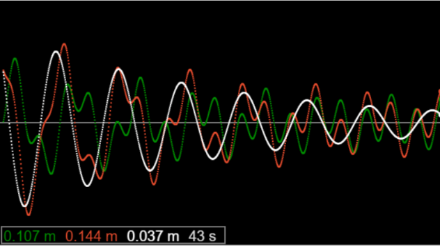
This illustration is from an earlier applet: the red and green curves correspond to different initial conditions, the white curve is the difference between the two, obviously exponentially decreasing, as can be verified analytically.
For the damped driven pendulum, the picture is more complicated. For curves corresponding to slightly different initial conditions will converge (except, for example, where, as mentioned above, varying the initial angle at a certain point switches from a final three-cycle to a two-cycle).
The Liapunov Exponent
For curves even with very small initial differences (say, 10-4 radians) separate exponentially, as is called the Lyapunov exponent.
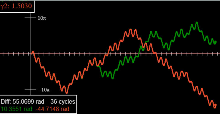
Bear in mind, though, that this is chaotic motion, the divergence is not as smooth as the convergence pictured above for the linear system. This graph is from our two-track applet.
Nevertheless, the (average) exponential nature can be discerned by plotting the logarithm of the difference against time:
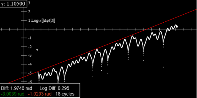
This is from our log difference applet. It is very close to Taylor’s fig 12.13. The red line slope gives the Lyapunov exponent.
(The red line has adjustable position and slope.)
Plotting Velocity against Time
As discussed in Taylor, further increase in the driving force beyond the chaotic threshold can lead to brief nonchaotic intervals, such as that containing the six cycle at 1.0845 illustrated above, but there are two long stretches of nonchaotic behavior in Taylor’s parameter range, from 1.1098 to 1.1482 and from 1.3 to 1.48.
In the stronger driving force range, the pendulum is driven completely around in each cycle, so plotting the position against time gives a “rounded staircase” kind of graph. Check this with the applet.
.
The solution is to plot velocity against time, and thereby discover that there is a repetition of the period doubling route to chaos at the upper end of this interval. Click to plot instead of
State-Space Trajectories
It can be illuminating to watch the motion develop in time in the two-dimensional state space (Equally called phase space.) See the State Space applet!
Now for a particle in a time-independent potential, specifying position and velocity at a given instant determines the future pathbut that is not the case here, the acceleration is determined by the phase of the driving force, which is time varying, so the system really needs three parameters to specify its subsequent motion.
That means the phase space is really three-dimensional, the third direction being the driving phase, or, equivalently, time, but periodic with the period of the driving force. In this three-dimensional space, paths cannot cross, at any point the future path is uniquely defined. Our two-dimensional plots are projections of these three-dimensional paths on to the plane.
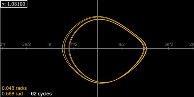
Here’s the 4-cycle at γ = 1.081, minus the first 20 cycles, to eliminate transients.
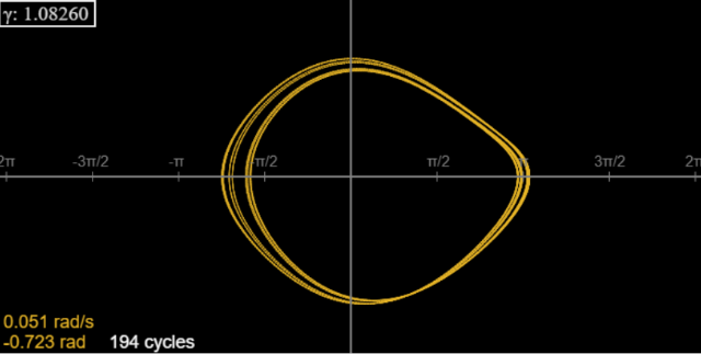
For γ = 1.0826, there is an 8-cycle. Run the applet for 40 cycles or so to get rid of transients, then look at the far-left end of the curve generated by running, say, to 200 cycles. It doesn’t look like there are 8 lines, but the outermost line and the two innermost lines are doubles (notice the thickness). You can check this with the applet, by pausing at the axis and noticing the position readout: there are 8 different values that repeat. (You don’t have to stop right on the axisyou can stop close to it, then use the step buttons to get there.)
For γ = 1.0830, the path is chaoticbut doesn’t look too different on this scale! Check it out with the applet. The chaos becomes more evident on further increasing γ. For γ =1.087 the pattern is “fattened” as repeated cycles differ slightly.
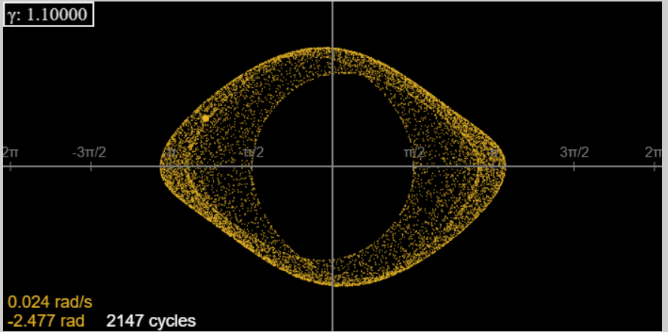
For further increase in γ, the orbital motion covers more territory: at γ = 1.1, here are the first three hundred or so cycles.
Plotting many orbits at high speed we find:
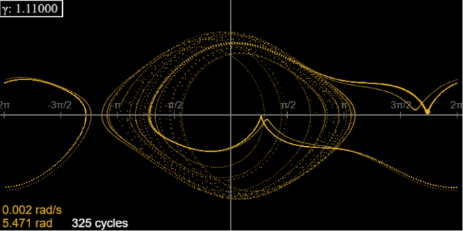
However, here the story gets complicated: it turns out that this chaotic series of orbits is in fact a transient, and after about 300 cycles the system skips to a 3-cycle, where it stays. In fact, we have reached a range of γ (approximately 1.1098 to 1.1482) where after initial transients (which can be quite long) the motion is not chaotic, but a 3-cycle.
Obviously, there is a lot to explore for this system! To get a better grasp of these complexities, we try a different approach, developed by Poincaré.
Poincaré Sections
Looking at the above pictures, as we go from a single orbit to successive period doublings and then chaos, the general shape of the orbit doesn’t change dramatically (until that final three-cycle). The interesting things are the doubling sequence, chaos, and attractorsperhaps we’re plotting too much information.
To focus on what’s essential, Poincaré plotted a single point from each cycle, this is now called a Poincaré section. To construct this, we begin with the t = 0 position, label it . Then add the point precisely one cycle later, and so onpoints one cycle apart, , etc. Now, knowing the position in state space is not enough information to plot the future orbitwe also need to know the phase of the driving force. But by plotting points one cycle in time apart, they will all see the same phase starting force, so the transformation that takes us from to just repeats in going from to etc.
To see these single points in the State Space applet, click “Show Red Dot”: on running, the applet will show one dot per cycle red.
Thinking momentarily of the full three-dimensional phase space, the Poincaré section is a cross-section at the initial phase of the driving cycle. We’ve added to the applet a red dot phase option, to find the Poincaré section at a different phase. Doing this a few times, and looking at the movement of the red dots, gives a fuller picture of the motion.
So the Poincaré section, on increasing γ through the doubling sequence (and always omitting initial transients) goes from a single point to two points, to four, etc.
To see all this a bit more clearly, the next applet, called Poincaré Section, shows only one dot per cycle, but has a phase option so you can look at any stage in the cycle.
Exercise: check this all out with the Poincaré applet! To see it well, click Toggle Origin/Scale, use the sliders to center the pattern, more or less, then scale it up. Run for a few hundred cycles, then click Hide Trace followed by Show Trace to get rid of transients.
Start with γ = 1.0826. The Poincaré section is eight points on a curve, at 1.0827 you can discern 16. By 1.0829, we have chaos, and the section has finite stretches of the curve, not just points. It looks very similar at 1.0831, butsurpriseat 1.0830 it’s a set of points (32?) some doubled. This tells us we’re in a minefield. There’s nothing smooth about chaos.
Apart from interruptions, as γ increases, the Poincaré section fills a curve, which then evolves towards the strange attractor shown by Taylor and others. Going from 1.090 in steps to 1.095, the curve evolves a second, closely parallel, branch. At 1.09650 the two branches are equal in length, then at 1.097 the lower branch suddenly extends a long curve, looks much the same at 1.100, then by 1.15 we recognize the emergence of the strange attractor.
But in fact this is a simplified narrative: there are interruptions. For example, at γ = 1.0960 there’s a 5-cycle, no chaos (it disappears on changing by 0.0001). And at 1.12 we’re in the 3-cycle interval mentioned earlier.
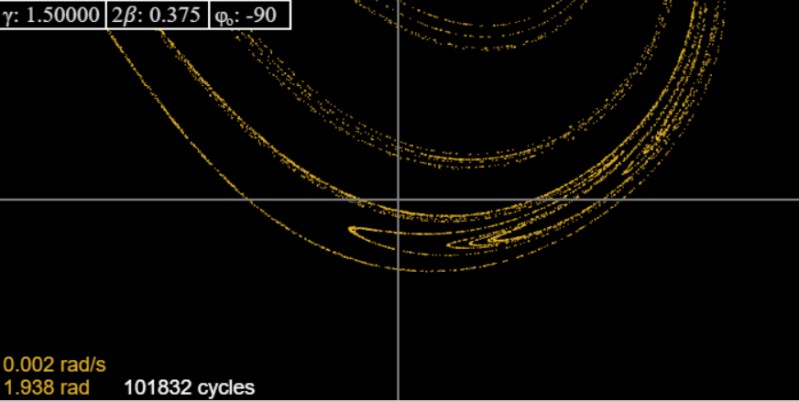
Anyway, the strange attractor keeps reappearing, and at 1.5 it looks like this:
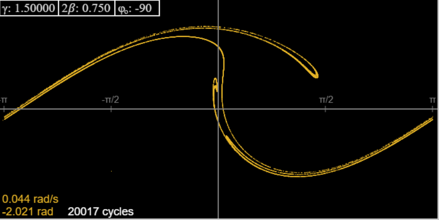
This looks rather thin compared to Taylor’s picture for the same γ: the reason is we have kept the strong damping.
Changing to we recover Taylor’s picture. Like him, we show here (from the applet) the attractor and successive magnifications of one part, to give some hint of the fractal structure:
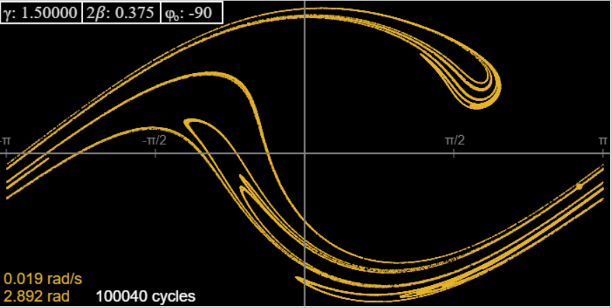
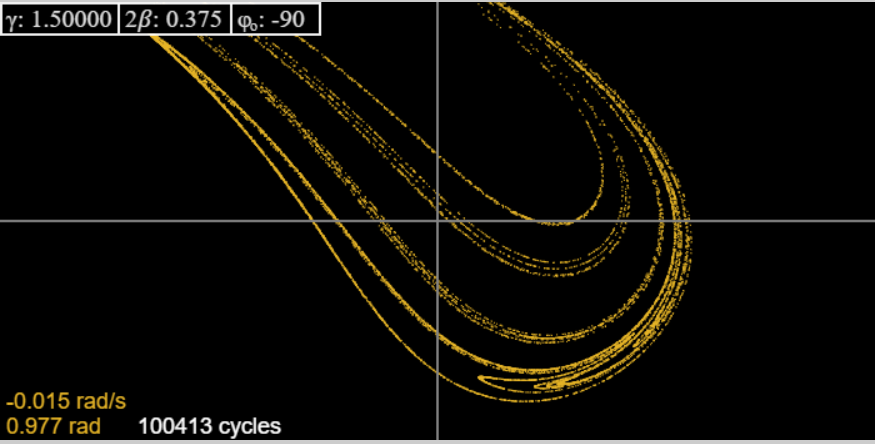
We have to admit that at the highest magnification Taylor’s picture is certainly superior to that generated by the applet, but does not contradict itactually, it reassures us that the applet is reliable up to the level of definition that is self-evident on looking at it.
Exercise: Use the last two applets to explore other regions of parameter space. What happens on varying the damping? Going from to the attractor has the same general form but is much narrower. Then go in 0.001 steps to 0.76. For some values you see the attractor, but for others a cycle, different lengths. There is a two-cycle from 0.76 to 0.766, then a four cycle, then at 0.78 back to a two-cycle, at 0.814 a one-cycle. If you up the driving strength, and the damping, you can find extremely narrow attractors.
Exercise: Baker and Gollub, Chaotic Dynamics, page 52, give a sequence of Poincaré sections at intervals for and You can check them (and intermediate ones) with the applet, and try to imagine putting them in a stack to visualize the full three-dimensional attractor!
Lyapunov Exponents and Dimensions of Strange Attractors
Scaling the Attractor
Looking at the strange attractor pictured in the previous section, we found that on magnifying a small part of it we saw the same kind of structure the attractor has as a whole: if we look at a attractor, with damping 0.75, there are long thin stretches, they end by looping over. We notice that halving the damping to 0.375 fattens the previously quasi-one-dimensional stretches and reveals complicated looping at several levels. (Remember that what we are looking at here is a Poincaré section of the attractor, the other dimension is periodic time (or driver phase, the same thing) so a curve here is a section of some sheet). If more computing power is used, going to smaller and smaller scales, it turns out that the magnified tiny part of the attractor looks much the same as the attractor. This kind of scale invariance is a characteristic of a fractal. A mysterious aspect of fractals is their dimensionality. Look at the strange attractor. There are no places where it solidly fills a stretch of two-dimensional space, this is clearer on going to greater and greater magnification: we see more and more one-dimensional structures, with no end, so it surely has dimension less than two, but greater than onehow do we make sense of that?
Fractals: the Cantor Set
To try to find a generalized concept of dimension of a set (i.e. not just an integer), we begin with perhaps the simplest example of a fractal, the Cantor set: take the numbers between 0 and 1, and cut out the middle third. You now have two strips of numbers, from 0 to 1/3, and from 2/3 to 1. For each of those strips, cut out the middle third. You now have four stripscut out the middle third of each of them (it might help to draw this). Do this forever. What’s left is the Cantor set. You can see this is scale invariant: after doing this many times, take one of the remaining tiny strips, what happens to it on continuing the process is identical (scaled down suitably) to what happened to the initial strip.
How big is this Cantor set? At each step, we cut the total length of line included by 2/3. Since (2/3)n goes to zero as n goes to infinity, it clearly has size zero, right? But clearly there’s more to the Cantor set than there is to a single point, or for that to matter a finite number of points. What about a countably infinite number of pointsfor example, the rational numbers between 0 and 1? Well, you can write them out in a list, ordered by increasing denominators, and for one denominator by increasing numerators. Then you can put them one by one into tiny intervals, goes into an interval of length 1/3 in an interval 2/3 in one of length in and so on, the total length of the infinite number of intervals being so all the rationals can be covered by an arbitrarily small set of intervals. Can we count in order the numbers in the Cantor set in the same way? The answer is no, and to see why think first about all the numbers between 0 and 1, rationals and irrationals. If you make an infinite list of them, I can show you missed some out: I just take your list and write down a decimal that differs from your nth number in the nth place. So we can’t put all the numbers in the interval in little boxes that add to zero, which is obvious anyway!
But now to the Cantor set: suppose we write all numbers between 0 and 1 using base 3, instead of the traditional base 10. That is, each number is a string of 0’s, 1’s and 2’s. Then the Cantor set is all those numbers that don’t have any 1’s, such as 0.2, 0.02202, etc. (Check this yourself.) But the number of these numbers is exactly the same as all the numbers between 0 and 1 in binary notation! So surely the Cantor set has dimension 1? (These infinities are tricky.)
The bottom line from the above argument is that we can plausibly argue both that the Cantor set has dimension 0, and that it has dimension 1. To understand and categorize fractals better, we need a working definition of dimension for fractals. One approach is the capacity dimension.
Dimensions: Capacity and Correlation
Suppose we cover the interval 0,1 with a set of small boxes, length there are clearly such boxes (assume it’s an integer). Now consider a subset of the numbers between 0 and 1, choose and find how many boxes are necessary to cover this subset. The capacity dimension is defined as
For simplicity, we choose so the necessary numbers of boxes to cover the Cantor set described in the previous section are 2, 4, 8… out of total numbers of boxes 3, 9, 27, … . Therefore
of course between 0 and 1. (There are many ways to define dimensionality of sets of numbersthis definition gives zero for a finite set of points, and one for all the numbers between 0 and 1, but also 1 for the set of rationals, which we’ve shown above can be covered by an infinite set of intervals of arbitrarily small total length.)
Another measure used is the correlation dimension, in which for a large number of points (such as our representation of the attractor) a correlation integral is defined as the total number of pairs of two points less than apart. For small this goes as a power and it turns out that in many cases is close to the capacity definition of the fractal dimension. (Grassberger and Procaccia.)
Time Development of Systems in Phase Space
Recall first that the state space or phase space we have been plotting is really a projection of the full orbit space into two dimensions, the third dimension necessary to predict future motion being the phase of the sine-wave driving force, so this is just time (although of course cyclic).
Suppose now we populate this three-dimensional space with many points, like a gas, each representing a driven damped pendulum. As time goes on the gas will flow, each gas atom’s path completely determined, and no two will ever be at the same point in this full space (except perhaps asymptotically at infinite time).
Take now a small volume, say a cube with sides parallel to the axes, containing many points. Consider first the undamped system: then Liouville’s Theorem (link to my lecture) tells us that as time goes on the cube will generally distort, but it will not change in volume. In other words, the gas of systems flows like an incompressible fluid. (Details of the derivation are given in the linked lecturebriefly, the motions of the sides in time come from the equations of motion, etc.)
However, if the system has dampingas ours doesthe same analysis leads to the conclusion that the volume the systems occupy in phase space (remember, this is now three-dimensional) shrinks at a rate determined by the damping. As a trivial example, think of undriven damped pendulathey will all tend to the low point rest position. Lightly driven pendula will go to a one-dimensional cycle.
We can prove this shrinkage from the equation of motion:
In the three-dimensional phase space, a pendulum’s position can be written in coordinates where the driving phase, between 0 and
The local phase space velocity can be written in terms of the coordinates (this is just the above equation rewritten!):
This is therefore the local velocity of the atoms of the gas (meaning the systems), and it is trivial to check that
This means that if we have a small sphere containing many points corresponding to systems (a “gas” of systems) then the volume of the (now distorting) sphere enclosing those points is decreasing in volume at an exponential rate
Relating this Picture to Lyapunov Exponents
Continuing to think about the development of a small sphere (containing many points corresponding to systems) in phase space, it will be moving along an orbit, but at the same time distorting, let’s say to an ellipsoid as an initial first approximation, and tumbling around. In the chaotic regime, we know it must be growing in some direction, at least on average (the rates will vary along the orbit) because we know that points initially close together separate on average at an exponential rate given by the first Lyapunov exponent, We’ll make the simplifying assumption that the ellipsoid has its axes initially varying in time as with From the result above we conclude that
We need to say something more about We’re taking it as defined by the growth rate of distance between trajectories after any initial transients but before the distance is comparable to the size of the system (finding this interval plausibly has been termed a “dark art”). We envision our initially small sphere of gas elongating and tumbling around as it moves along. Hopefully its rate of elongation correlates well with what we actually measure, that is, the rate of growth of net displacement, the coordinate separation of two initially close orbits, which we plot and approximately fit with an exponential,
For the pendulum, the direction is just time, not scaled, so Then necessarily to satisfy the damping equation.
So taking a local (in phase space) collection of systems, those inside a given closed surface, like a little sphere, and following their evolution in time in the chaotic regime, the sphere will expand in one direction; a direction, however, that varies with time, but contract or stay constant in the other directions. As the surface grows this gets more complicated because it’s confined to a finite total phase space. And it continues to expand at the same rate as time goes on, so the continual increase in surface must imply tighter and tighter foldings to stay in the phase space. And this is what the strange attractor looks like.
A Fractal Conjecture
In 1979, Kaplan and Yorke conjectured that the dimensionality of the strange attractor followed from the Lyapunov exponents taking part in its creation. In our casethe driven damped pendulumthere are only two relevant exponents, and
A plausibility argument is given in Baker and Gollub’s book, Chaotic Dynamics. They define a Lyapunov dimension of the attractor by
exactly analogous to the definition of capacity dimension in the previous section.
Now, as time passes a small square element will have its area multiplied by a factor (No scaling takes place in the third (time) direction.) At the same time, they argue that the length unit changes as Then is the area divided by the shrinking basic area The differential of is that of is so their argument gives
The Lyapunov applet is designed to measure by tracking separation of initially close trajectories. Try it a few times: it becomes clear that there is considerable uncertainty in this approach. Given follows from There are various ways to assign a dimension to the attractor, such as the capacity and correlation dimensions mentioned above. Various attempts to verify this relationship have been made, but the uncertainties are considerable, and although results seem to be in the right ballpark, the results are off by ten or twenty percent typically. It seems there is work still to be done on this fascinating problem.
Recommended reading: chapter 5 of Baker and Gollub, Chaotic Dynamics. The brief discussion above is based on their presentation.