6. Hamilton’s Equations
Michael Fowler
A Dynamical System’s Path in Configuration Space, State Space and Phase Space
Configuration Space and State Space
The story so far: For a mechanical system with degrees of freedom, the spatial configuration at some instant of time is completely specified by a set of variables we'll call the ’s. The -dimensional space is (naturally) called configuration space. It’s like a freeze frame, a snapshot of the system at a given instant. Subsequent time evolution from that state is uniquely determined if we're also given the initial velocities .
The set of and together define the state of the system, meaning both its configuration and how fast it’s changing, therefore fully determining its future (and past) as well as its present. The -dimensional space spanned by is the state space.
The system’s time evolution is along a path in configuration space parameterized by the time That, of course, fixes the corresponding path in state space, since differentiating the functions along that path determines the
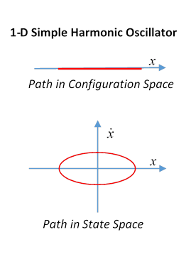 Trivial one-dimensional examples of these spaces are
provided by the one-dimensional simple harmonic oscillator, where configuration
space is just the axis, say, the state space is the plane, the system’s time path in the state
space is an ellipse.
Trivial one-dimensional examples of these spaces are
provided by the one-dimensional simple harmonic oscillator, where configuration
space is just the axis, say, the state space is the plane, the system’s time path in the state
space is an ellipse.
For a stone falling vertically down, the configuration space is again a line, the path in the state space is parabolic,
Exercise: Sketch the paths in state space for motions of a pendulum, meaning a mass at the end of a light rod, the other end fixed, but free to rotate in one vertical plane. Sketch the paths in coordinates.
In principle, the system’s path through configuration space can always be computed using Newton’s laws of motion, but in practice the math may be intractable. As we’ve shown above, the elegant alternative created by Lagrange and Hamilton is to integrate the Lagrangian
along different paths in configuration space from a given initial state to a given final state in a given time: as Hamilton proved, the actual path followed by the physical system between the two states in the given time is the one for which this integral, called the action, is minimized. This minimization, using the standard calculus of variations method, generates the Lagrange equations of motion in , and so determines the path.
Notice that specifying both the initial ’s and the final ’s fixes variables. That’s all the degrees of freedom there are, so the motion is completely determined, just as it would be if we’d specified instead the initial ’s and ’s.
Phase Space
More Natural Variables...
Newton wrote his equation of motion not as force equals mass times acceleration, but as force equals rate of change of momentum. Momentum, mass times velocity, is the natural "quantity of motion" associated with a time-varying dynamical parameter. It is some measure of how important that coordinate's motion is to the future dynamical development of the system.
Hamilton recast Lagrange's equations of motion in these more appropriate variables , positions and momenta, instead of . The 's and 's are called phase space coordinates.
So phase space is the same identical underlying space as state space, just with a different set of coordinates. Any particular state of the system can be completely specified either by giving all the variables or by giving the values of all the .
By the way, the are the sets of variables used in quantum mechanics, and their noncommutativity yields a quantum measure in phase space, from which follows an absolute number for entropy..
Going From State Space to Phase Space
Now, the momenta are the derivatives of the Lagrangian with respect to the velocities, . So, how do we get from a function of positions and velocities to a function of positions and the derivatives of that function with respect to the velocities?
How It's Done in Thermodynamics
To see how, we'll briefly review a very similar situation in thermodynamics: recall the expression that naturally arises for incremental energy, say for the gas in a heat engine, is
where is the entropy and is the temperature. But is not a handy variable in real life -- temperature is a lot easier to measure! We need an energy-like function whose incremental change is some function of rather than The early thermodynamicists solved this problem by introducing the concept of the free energy,
so that This change of function (and variable) was important: the free energy turns out to be more practically relevant than the total energy, it's what's available to do work.
So we've transformed from a function to a function (ignoring , which are passive observers here).
Math Note: the Legendre Transform
The change of variables described above is a standard mathematical routine known as the Legendre transform. Here’s the essence of it, for a function of one variable.
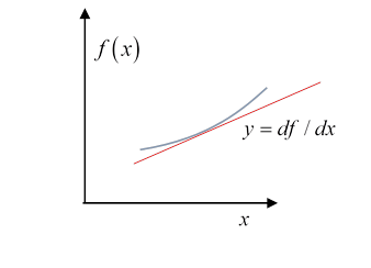
Suppose we have a function that is convex, which is math talk for it always curves upwards, meaning is positive. Therefore its slope, we’ll call it
,
is a monotonically increasing function of . For some physics (and math) problems, this slope , rather than the variable is the interesting parameter. To shift the focus to , Legendre introduced a new function, , defined by
The function is called the Legendre transform of the function .
To see how they relate, we take increments:
(Looking at the diagram, an increment gives a related increment as the slope increases on moving up the curve.)
From this equation,
Comparing this with it’s clear that a second application of the Legendre transformation would get you back to the original . So no information is lost in the Legendre transformation— in a sense contains and vice versa.
Hamilton's Use of the Legendre Transform
From State Space to Phase Space
We have the Lagrangian and Hamilton's insight that these are not the best variables, we need to replace the Lagrangian with a closely related function (like going from the energy to the free energy), that is a function of the (that's not going to change) and, instead of the 's, the 's, with . This is exactly a Legendre transform like the one from discussed above.
The new function is
from which
analogous to This new function is of course the Hamiltonian.
Checking that We Can Eliminate the
We should check that we can in fact write
as a function of just the variables , with all trace of the ’s eliminated. Is this always possible? The answer is yes.
Recall the ’s only appear in the Lagrangian in the kinetic energy term, which has the general form
where the coefficients depend in general on some of the ’s, but are independent of the velocities, the ’s. Therefore, from the definition of the generalized momenta,
and we can write this as a vector-matrix equation,
.
That is, is a linear function of the ’s. Hence, the inverse matrix will give us as a linear function of the , and then putting this expression for the into the Lagrangian gives the Hamiltonian as a function only of the and the , that is, the phase space variables.
The matrix is always invertible because the kinetic energy is positive definite (as is obvious from its Cartesian representation) and a symmetric positive definite matrix has only positive eigenvalues, and therefore is invertible.
Hamilton’s Equations
Having finally established that we can write, for an incremental change along the dynamical path of the system in phase space,
we have immediately the so-called canonical form of Hamilton’s equations of motion:
Evidently going from state space to phase space has replaced the second order Euler-Lagrange equations with this equivalent set of pairs of first order equations.
A Simple Example
For a particle moving in a potential in one dimension,
Hence
Therefore
(Of course, this is just the total energy, as we expect.)
The Hamiltonian equations of motion are
So, as we’ve said, the second order Lagrangian equation of motion is replaced by two first order Hamiltonian equations. Of course, they amount to the same thing (as they must!): differentiating the first equation and substituting in the second gives immediately that is, the original Newtonian equation (which we derived earlier from the Lagrange equations).