1. Introductory Statics: the Catenary and the Arch
Michael Fowler
The Catenary
What is the shape of a chain of small links hanging under gravity from two fixed points (one not directly below the other)? The word catenary (Latin for chain) was coined as a description for this curve by none other than Thomas Jefferson! Despite the image the word brings to mind of a chain of links, the word catenary is actually defined as the curve the chain approaches in the limit of taking smaller and smaller links, keeping the length of the chain constant. In other words, it describes a hanging rope. A real chain of identical rigid links is then a sort of discretization of the catenary.
We’re going to analyze this problem as an introduction to the calculus of variations. First, we’re going to solve it by a method you already know and lovejust (mentally) adding up the forces on one segment of the rope. The tension is pulling at both ends, the segment’s weight acts downwards. Since it’s at rest, these three forces must add to zero. We’ll show that writing down the balance of forces equation gives sufficient information to find the curve of the chain , meaning height above ground as a function of horizontal position . So we understand the mechanics of the problem.
But next we take a completely different approach: we assume the shape of the chain is described by an arbitrary function , required to go between the two fixed endpoints and to have total length equal to that of the (assumed inextensible) rope, and we work out its gravitational energy. We know, of course, that the true curve the rope settles into will be the one of minimum potential energy. The rope is at the bottom of a multidimensional potential well. This means that any slight variation from this minimum shape will only affect the potential energy to second order, in precise analogy with a slight change in position of a particle at the minimum point of a potential energy well.
So the technique, called the Calculus of Variations, is to find where the derivative of the potential energy with respect to variations of this curve becomes zerothat will be the minimum energy configuration we’re looking for. Conceptually, this is a lot more complicated than ordinary differentiation with respect to one, or a few, variables. We’re varying a whole function. This is why it’s was worth solving the problem using traditional statics to begin withit reassures us that the variational approach works.
A Cambridge mathematician, William Whewell, famously stated in unconscious rhyme,
And so no force, however great,
can pull a string, however fine,
into a horizontal line,
that shall be absolutely straight.
(Trivial fact: Whewell had a way with words—he even invented some of the words you use every day, for example the words scientist, physicist, ion, cathode, anode, dielectric, and lots more.)
A Tight String
Let’s take the hint and look first at a piece of uniform string at rest under high tension between two points at the same height, so that it’s almost horizontal.
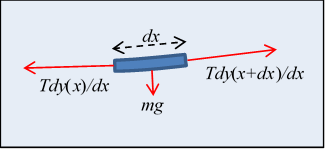
Each little bit of the string is in static equilibrium, so the forces on it balance. First, its weight acting downwards is , being the uniform mass per unit length. Second, the tension forces at the two ends don’t quite balance because of the small change in slope.
Representing the string configuration as a curve , the balance of forces gives
so , and , taking the lowest point of the string as the origin.
So the curve is a parabola (but keep reading!).
Not So Tight
In fact, there are hidden approximations in the above analysisfor one thing, we’ve assumed that the length of string between and is but it’s really where the distance parameter is measured along the string. Second, we took the tension to be nonvarying. That’s a pretty good approximation for a string that’s almost horizontal, but think about a string a meter long hanging between two points 5 cm apart, and it becomes obvious that both these approximations are only good for a near-horizontal string.
Obviously, with the string nearly vertical, the tension is balancing the weight of string below it, and must be close to zero at the bottom, increasing approximately linearly with height. Not to mention, it’s clear that this is no parabola, the two sides are very close to parallel near the top. The constant approximation is evidently no goodbut Whewell solved this problem exactly, back in the 1830’s.
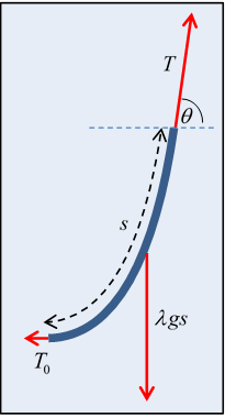
What he did was to work with the static equilibrium equation for a finite length of string, one end at the bottom.
If the tension at the bottom is , and at a distance s away, measured along the string, the tension is , and the string’s angle to the horizontal there is (see diagram), then the equilibrium balance of force components is
,
from which the string slope
where we have introduced the constant which sets the length scale of the problem.
So we now have an equation for the catenary, in terms of distance along the string. What we want, though is an equation for vertical position in terms of horizontal position the function for the chain.
Now we’ve shown the slope is
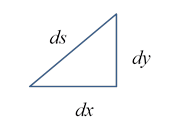
and the infinitesimals are related by so putting these equations together
that is,
Taking the square root and rearranging
which can be integrated immediately with the substitution
,
to give just
,
which integrates trivially to , with a constant of integration, or
,
choosing the origin at , which makes .
But of course what we want is the curve shape , not . We need to eliminate in favor of That is, we need to write as a function of , then substitute .
Recall one of our first equations was for the slope and putting that together with gives
,
integrating to
.
This is the desired equation for the catenary curve
We’ve dropped the possible constant of integration, which is just the vertical positioning of the origin.
Question: is this the same as the curve of the chain in a suspension bridge?
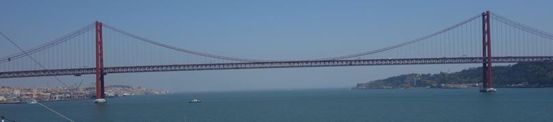
(Notice the vertical ropes are uniformly spaced horizontally.)
Ideal Arches
Now let’s consider some upside-down curves, arches. Start with a Roman arch, an upside-down U.
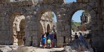
Typically, Roman arches are found in sets like this, but let’s consider one free standing arch. Assume it’s made of blocks having the same cross-section throughout. What is the force between neighboring blocks? We’ll do an upside-down version of the chain force analysis we just did.
Equating the pressure forces on the arch segment colored dark in the figure, we see pressure on the lowest block in the segment must have a horizontal component, to balance the forced at the top point, so the cement between blocks is under shear stress, or, for no cement, there’s a strong sideways static frictional force. (So a series of arches, as shown in the photograph above, support each other with horizontal pressure.)
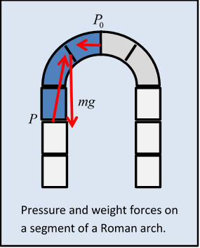
A single Roman arch like this is therefore not an ideal designit could fall apart sideways.
Let’s define an ideal arch as one that doesn’t have a tendency to fall apart sideways, outward or inward. This means no shear (sideways) stress between blocks, and that means the pressure force between blocks in contact is a normal forceit acts along the line of the arch. That should sound familiar! For a hanging string, obviously the tension acts along the line of the string.
Adding to our ideal arch definition that the blocks have the same mass per unit length along the entire arch, you can perhaps see that the static force balance for the arch is identical to that for the uniform hanging string, except that everything’s reversedthe tension is now pressure, the whole thing is upside down.
Nevertheless, apart from the signs, the equations are mathematically identical, and the ideal arch shape is a catenary. Of course, some actual constructed arches, like the famous one in St. Louis, do not have uniform mass per unit length (It’s thicker at the bottom) so the curve deviates somewhat from the ideal arch catenary.
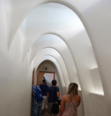
Here’s a picture of catenary archesthese arches are in Barcelona, in a house designed by the architect Gaudi.
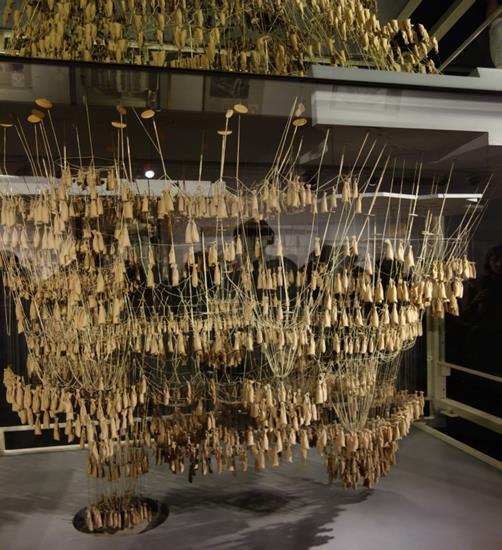
In fact, Gaudi designed a church in Barcelona using a web of strings and weights to find correct shapes for the archeshe placed a large horizontal mirror above the strings, so looking in the mirror he could see what the actual right-way-up building would look like!The lower image shows how he did it. (This model is in the church.)